CBSE Class 12 Marking Scheme 2022 for Applied Maths Term 2
Finished viewing? Save it for later —
Download CBSE Class 12 Marking Scheme 2022 for Applied Maths Term 2 (PDF · 6 pages)About CBSE Class 12 Marking Scheme 2022 for Applied Maths Term 2
CBSE Class 12 Marking Scheme 2022 for Applied Maths Term 2 is available here for free download. Published by CBSE for Class 12, this marking scheme can be viewed online or downloaded as a PDF (6 pages). Candidates preparing for Class 12 can use CBSE Class 12 Marking Scheme 2022 for Applied Maths Term 2 to understand the exam pattern, the type of questions asked, and the overall difficulty level.
Frequently Asked Questions
How can I download CBSE Class 12 Marking Scheme 2022 for Applied Maths Term 2?
Open this page and click the Download button to save CBSE Class 12 Marking Scheme 2022 for Applied Maths Term 2 as a PDF. It is completely free on AglaSem Docs.
Is CBSE Class 12 Marking Scheme 2022 for Applied Maths Term 2 free to download?
Yes. CBSE Class 12 Marking Scheme 2022 for Applied Maths Term 2 can be viewed online and downloaded as a PDF free of cost on AglaSem Docs.
How many pages does CBSE Class 12 Marking Scheme 2022 for Applied Maths Term 2 have?
CBSE Class 12 Marking Scheme 2022 for Applied Maths Term 2 contains 6 pages, which you can read online or download together as a single PDF.
Where can I find more Class 12 study material?
You can find more Class 12 question papers, sample papers, syllabus, and answer keys on AglaSem Docs.
CBSE Class 12 Marking Scheme 2022 for Applied Maths Term 2 – Text
Read the full text of this marking scheme below — useful to quickly search, copy and reference the content online without downloading the PDF.
📄 View text version (6 pages)
Page 1
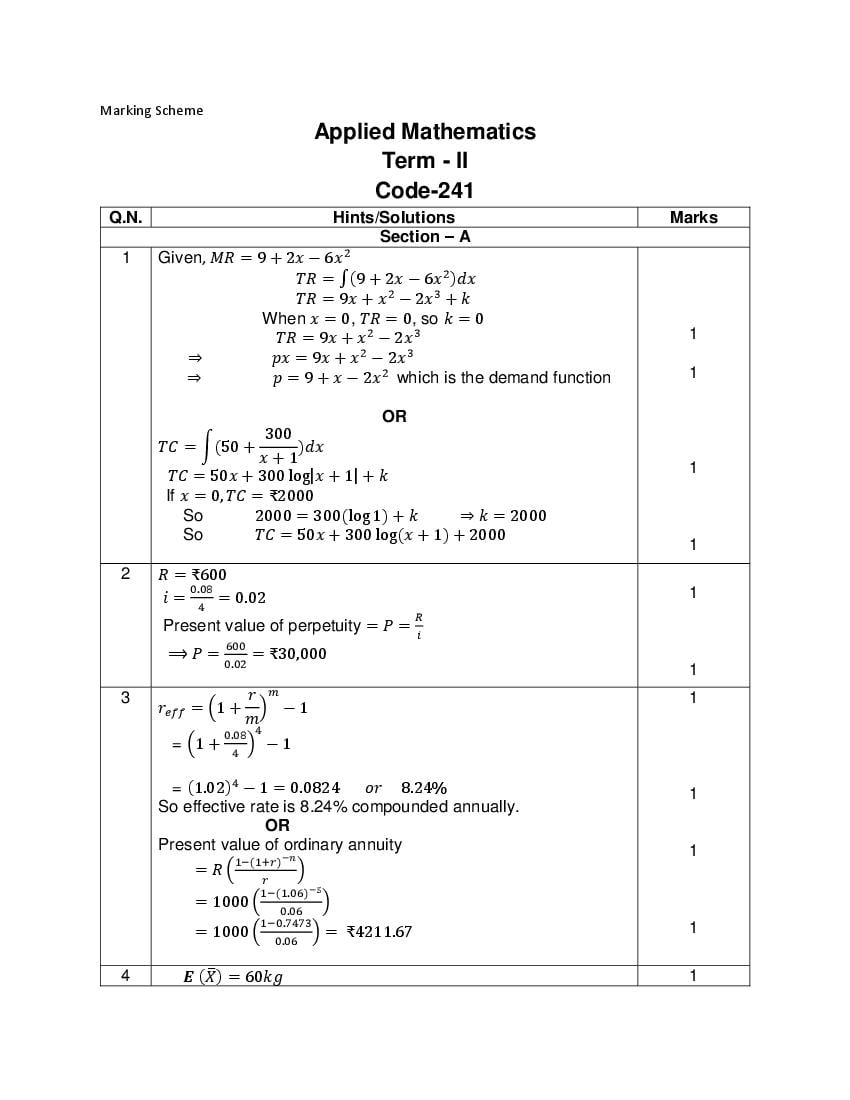
Applied Mathematics
Term - II
Code-241
Q.N. Hints/Solutions Marks
Section – A
2
1 Given, 𝑀𝑅 = 9 + 2𝑥 − 6𝑥
𝑇𝑅 = ∫(9 + 2𝑥 − 6𝑥 2 )𝑑𝑥
𝑇𝑅 = 9𝑥 + 𝑥 2 − 2𝑥 3 + 𝑘
When 𝑥 = 0, 𝑇𝑅 = 0, so 𝑘 = 0
𝑇𝑅 = 9𝑥 + 𝑥 2 − 2𝑥 3 1
⇒ 𝑝𝑥 = 9𝑥 + 𝑥 2 − 2𝑥 3
⇒ 𝑝 = 9 + 𝑥 − 2𝑥 2 which is the demand function 1
OR
300
𝑇𝐶 = ∫(50 + )𝑑𝑥
𝑥+1
𝑇𝐶 = 50𝑥 + 300 log|𝑥 + 1| + 𝑘 1
If 𝑥 = 0, 𝑇𝐶 = ₹2000
So 2000 = 300(log 1) + 𝑘 ⇒ 𝑘 = 2000
So 𝑇𝐶 = 50𝑥 + 300 log(𝑥 + 1) + 2000
1
2 𝑅 = ₹600
0.08 1
𝑖 = 4 = 0.02
𝑅
Present value of perpetuity = 𝑃 =
𝑖
600
⟹ 𝑃 = 0.02 = ₹30,000
1
3 𝑟 𝑚 1
𝑟𝑒𝑓𝑓 = (1 + ) −1
𝑚
0.08 4
= (1 + ) −1
4
= (1.02)4 − 1 = 0.0824 𝑜𝑟 8.24% 1
So effective rate is 8.24% compounded annually.
OR
Present value of ordinary annuity 1
1−(1+𝑟)−𝑛
= 𝑅( )
𝑟
1−(1.06)−5
= 1000 ( )
0.06
1−0.7473 1
= 1000 ( ) = ₹4211.67
0.06
4 𝑬 (𝑋̅) = 60𝑘𝑔 1
Page 2
Standard deviation of 𝑋̅ = 𝑆𝐸 (𝑋̅) = = 6 = 1.5 𝑘𝑔
√ 𝑛
1
5 Year Y 3 yearly 3 yearly moving 1M for
moving total average(Trend) 3-yearly
2016 25 --- --- moving
2017 30 87 29 totals
2018 32 102 34
2019 40 117 39 1M for
2020 45 135 45 3-yearly
2021 50 --- --- moving
average
6
Corner Point Z=3x+2y
P (2, 2) 10 1
Q (3, 0) 9
The smallest value of Z is 9. Since the feasible region is
unbounded, we draw the graph of 3𝑥 + 2𝑦 < 9. The resulting
open half plane has points common with feasible region,
therefore Z = 9 is not the minimum value of Z. Hence the optimal 1
solution does not exist.
Section –B
7 Substituting, 𝑝0 = ₹48 in 𝑝 = 𝑥 2 + 4𝑥 + 3
We get 𝑥0 = 5 1
𝑥
𝑃𝑆 = 𝑝0 𝑥0 − ∫0 0 𝑔(𝑥)𝑑𝑥
5 1
= 48 × 5 − ∫0 (𝑥 2 + 4𝑥 + 3)𝑑𝑥
𝑥3 5 1
= 240 − [ 3 + 2𝑥 2 + 3𝑥] = ₹133.33
0
Page 3
Year Quarters Y 4-Quarterly 4 Quarterly 1
1 2 for
Moving Total Moving average
(Centered) 4 quarterly
moving
𝑄1 12 --
totals
𝑄2 14 --
2018 𝑄3 18 64 16.75
𝑄4 20 70 17.75
72
𝑄1 18 18.25
74
2019 𝑄2 16 18.75
76 1
𝑄3 20 85 20.125 1 2 for 4
𝑄4 22 93 22.25
Quarterly
𝑄1 27 103 24.50 moving
2020 𝑄2 24 117 27.5 average
𝑄3 30 -- (Centered)
𝑄4 36 --
The trend value are given by 4 quarterly centered moving
average.
𝑶𝑹
𝑌𝑒𝑎𝑟 𝑌 𝑋 𝑋2 𝑋𝑌
= 𝑌𝑒𝑎𝑟 − 2017
2014 26 -3 9 -78
2015 26 -2 4 -52
2016 44 -1 1 -44
2017 42 0 0 0
2018 108 1 1 108
2019 120 2 4 240
2020 166 3 9 498 1
∑ 𝑌 = 532 ∑ 𝑋 2 = 28 ∑ 𝑋𝑌
= 672
∑𝑌 532 ∑ 𝑋𝑌 672
𝑎 = 𝑛 = 7 = 76, 𝑏 = ∑ 𝑋 2 = 28 = 24
1
𝑌𝑐 = 𝑎 + 𝑏𝑋, 𝑌𝑐 = 76 + 24𝑋
1
Estimated sales = 𝑌𝑐 for 2023 = 76 + 24 × 6 = ₹220 lacs
9 Define Null hypothesis 𝐻0 and alternate hypothesis 𝐻1 as follows:
𝐻0 : 𝜇 = 0.50 𝑚𝑚
𝐻1 : 𝜇 ≠ 0.50 𝑚𝑚 1
Page 4
have 1
𝑋̅−𝜇 0.53−0.50
𝑡 = 𝑆 √𝑛 − 1 = 0.03 × 3 = 3
Since the calculated value of 𝑡 = 3 does not lie in the internal
−𝑡0.025 to 𝑡0.025 i.e., -2.262 to 2.262 for 10-1= 9 degree of freedom
So we Reject 𝐻0 at 0.05 level. Hence we conclude that machine 1
is not working properly.
10
We know
1
𝐹𝑉 𝑛
CAGR=[( 𝐼𝑉 ) − 1] × 100, where, IV= Initial value of investment
FV=Final value of investment 1
1 1
25000 𝑛 5 𝑛
⇒ 8.88 = [( ) − 1] × 100 ⇒ 0.0888 = ( ) − 1
15000 3
1
1
⇒ 1.089 = (1.667)𝑛
1
⇒ 𝑛 log(1.667) = log(1.089) ⇒ 𝑛(0.037) = 0.2219
1
⇒ 𝑛 = 5.99 ≈ 6 𝑦𝑒𝑎𝑟𝑠
Section –C
11 Let the company produces 𝑥 and 𝑦 gallons of alkaline solution
and base oil respectively, also let 𝐶 be the production cost.
Min 𝐶 = 200𝑥 + 300𝑦
subject to constraints:
𝑥 + 𝑦 ≥ 3500 … . (1)
𝑥 ≥ 1250 … . (2) 1
1
2𝑥 + 𝑦 ≤ 6000. . . (3) 2
𝑥, 𝑦 ≥ 0
1
1
2
Corner Points 𝑪 = 𝟐𝟎𝟎𝒙 + 𝟑𝟎𝟎𝒚
P(1250, 2250) ₹9,25,000
Page 5
R(2500, 1000) ₹8,00,000
Minimum cost is 8,00,000 when 2500 gallons of alkaline
solutions & 1000 gallons of base oil are manufactured. 1
12 The amount of sinking fund S at any time is given by
(1+𝑖)𝑛 −1 1
𝑆 = 𝑅[ ]
𝑖
Where 𝑅 = 𝑃𝑒𝑟𝑖𝑜𝑑𝑖𝑐 𝑝𝑎𝑦𝑚𝑒𝑛𝑡, 𝑖 = 𝐼𝑛𝑡𝑒𝑟𝑒𝑠𝑡 𝑝𝑒𝑟 𝑝𝑒𝑟𝑖𝑜𝑑,
𝑛 = 𝑛𝑢𝑚𝑏𝑒𝑟 𝑜𝑓 𝑝𝑎𝑦𝑚𝑒𝑛𝑡𝑠
𝑆= Cost of machine – Salvage value
= 50,000-5000 = ₹45,000
8%
𝑖 = 4 = 0.02
(1+.02)40 −1 1
⟹ 45000 = 𝑅 [ ] 1
0.02 2
2.208−1
⟹ 45000 = 𝑅 [ 0.02 ]
900
⟹ 𝑅 = 1.208 ⟹ 𝑅 = ₹745.03 1
1
2
13. Amortized Amount i.e., P= Cost of house-Cash down payment
P= 15,00,000 – 4,00,000 = ₹11,00,000
0.09
𝑖 = 12 = 0.0075
1
𝑛 = 10 × 12 = 120
𝑃
EMI = 𝑅 = 𝑎 ,
𝑛¬𝑖
𝑃×𝑖 1
𝑅 = 1−(1+𝑖)−𝑛
11,00,000 ×0.0075 8250
= 1−(1.0075)−120 = 1−0.4079 1
8250
= 0.5921 = ₹13933.5
Total interest paid = 𝑛𝑅 − 𝑅 = 13933.5 × 120 − 11,00,000 1
=₹5,72,020
OR
Face value of bond, F = ₹2000
Redemption value C = 1.05 × 2000 = ₹2100
Nominal rate =8% 1
𝑅 = 𝐶 × 𝑖𝑑 = 2000 × 0.08 = ₹160 1
2
Number of periods before redemption i.e., n = 10
Annual yield rate, 𝑖 =10% or 0.1
1−(1+𝑖)−𝑛 1
Purchase price 𝑉 = 𝑅 [ ] + 𝐶(1 + 𝑖)−𝑛 1
𝑖
1−(1+0.1)−10 2
= 160 [ ] + 2100(1 + 0.1)−10
0.1
= 160 × 6.14 + 2100 × 0.3855
= 982.4 + 809.6 = 1792
Page 6
14 Case Study
a) 𝑑𝑥 𝑑𝑥
∵ ∝ 𝑥, ∴ = −𝑘𝑥
𝑑𝑡 𝑑𝑡
𝑑𝑥 1
⇒ ∫ 𝑥 = ∫ −𝑘 𝑑𝑡 ⇒ log 𝑥 = −𝑘𝑡 + 𝑐
⇒ 𝑥 = 𝑒 −𝑘𝑡+𝐶 ⇒ 𝑥 = 𝜆𝑒 −𝑘𝑡
Let 𝑥 = 𝑥0 𝑎𝑡 𝑡 = 0
∵ 𝑥0 = 𝜆 ⇒ 𝑥 = 𝑥0 𝑒 −𝑘𝑡 where 𝑥0 = original quantity 1
b) 𝑥 = 𝑥0 𝑒 −𝑘𝑡 … . . (1)
𝑥
Now, 20 = 𝑥0 𝑒 −5𝑘 (∵ half life = 5 hours)
1
1
⇒ 𝑒 −5𝑘 = 2 ⇒ 𝑒 𝑘 = 2 5
1
The quantity of propofol needed in a 50 years adult after
2 hours = 50 × 3 = 150 mg ⇒ 150 = 𝑥0 𝑒 −2𝑘 [ using… (1)]
⇒ 𝑥0 = 150 𝑒 2𝑘 ⇒ 𝑥0 = 150 (𝑒 𝑘 )2
1
⇒ 𝑥0 = 150(25 )2 = 150 × 1.3195 = 197.93 mg 1
Document Details
| Board / Org | CBSE |
| Exam | Class 12 |
| Type | Solution |
| Pages | 6 |
| Language | english |
| Updated | 30 Apr 2026 |